컴퓨팅 설계

Computing Services, Server Types, and Sizing

Choosing the Right Compute Service for Your Workload

The computing service specifications provided by Samsung Cloud Platform are as follows.

Note: You can check the latest server types by visiting the website below. Virtual Server : https://cloud.samsungsds.com/serviceportal/services/compute/virtualServer.html GPU Server : https://cloud.samsungsds.com/serviceportal/services/compute/gpuServer.html Bare Metal Server : https://cloud.samsungsds.com/serviceportal/services/compute/baremetal.html

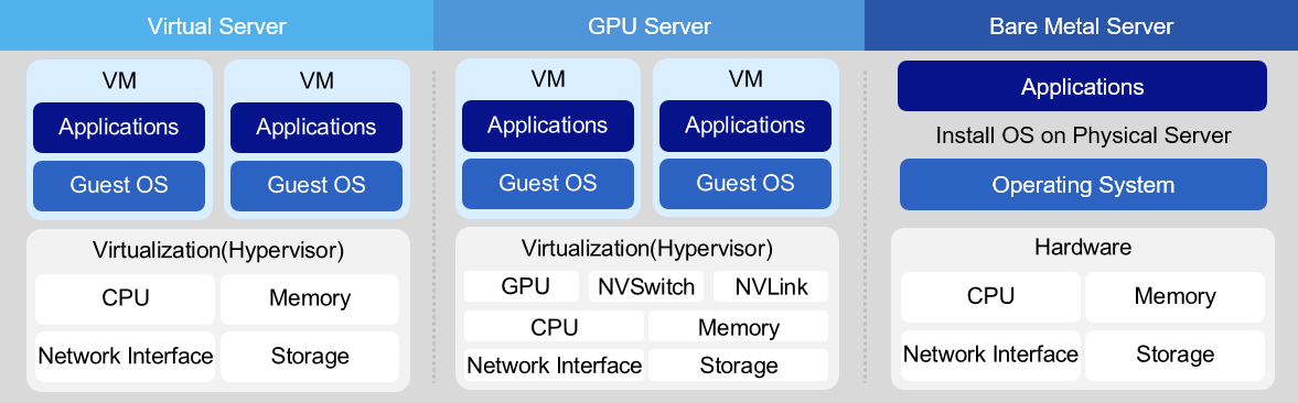
• Virtual Server Virtual Server provides a Standard (s1) type of up to 16 vCores and a High Capacity (h2) type of 24 vCores or more. The Standard type uses an Intel Ice Lake CPU, and 1vCore/2GB is the minimum specification. From 2 vCore up to 16 vCore, they are offered in CPU:Memory ratios of 1:2, 1:4, 1:8, and 1:16. The High Capacity type uses Intel Sapphire Rapids CPUs and offers CPU:Memory combinations in 1:2, 1:4, 1:8, and 1:12 ratios, ranging from 24 vCore to 128 vCore. The operating systems include RHEL, Ubuntu, Alma, Rocky, Oracle Linux, and Windows Server, and you can configure Kubernetes images, Data Service Console images, and so on. Virtual Server can be utilized for various purposes, such as development, testing, and Application execution, depending on the user’s computing needs.

• Bare Metal Server A Bare Metal Server is a high‑performance cloud computing service that does not use virtualization technology and allocates physically isolated computing resources such as CPU and memory exclusively. The 3rd generation service using Intel Sapphire Rapids is currently available. The CPU:Memory combinations for the provided server types are available in 1:4, 1:8, and 1:16. The default Internal Disk for the OS is 480GB2 for 16 vCore, 960GB2 for 32 vCore, and 1.92TB*2 for 96/128 vCore. Bare Metal Servers are suitable for workloads requiring high capacity and high performance, such as real-time systems, HPC (High Performance Computing), and servers requiring heavy I/O usage. Additionally, you can leverage the Multi-Attach feature to configure databases that require Active-Active high availability.

Server Sizing

After selecting a computing service suitable for the workload, you must determine the server specifications and quantity based on availability and performance requirements.

While determining server specifications and quantities was a critical process in on-premises environments, in cloud environments, it becomes a flexible task that can be changed at any time.

This is because adjustments can be made later, even if there is a difference between the initially set specifications and the actual required specifications.

Nevertheless, server sizing is important because we must calculate the workload operating cost (monthly fee) in the cloud and, based on that, derive the TCO (Total Cost of Ownership) compared to on‑premises deployment.

To estimate the hardware scale of an information system, the following three methodologies can be considered.

Calculation formulas and reference methods estimate the resource usage of servers deployed on the cloud by extracting various metrics.

Generally, cloud capacity planning identifies the capacity balance point by adjusting through simulation methods or operations.

However, sizing is often required for reasons such as cost estimation or proposals.

The formula-based calculation method can provide objective capacity design criteria because it calculates server capacity using various metrics.

Web/WAS CPU Sizing Based on Formula Calculation

First, calculate the CPU capacity of the Web/WAS server using the formula.

• Concurrent users
  Concurrent users refer to users who simultaneously use software or a system on a network, and are typically defined based on a session (from business service request to service termination). The calculation is based on the CPU cores utilized by the existing information system server. If the hierarchical configuration of the existing server changes, we compute a correction factor taking load balancing into account. First, estimate the total number of system users. The total number of users usually refers to the total users registered in the system, but generally refers to users with access permissions. However, in the case of the web, since unspecified users can access it, estimation is required. Next, calculate the number of concurrent users as a specific percentage of the total number of users. A connected user is a user who is online and may generate transactions or operations, or may simply be connected. Finally, you can estimate the number of concurrent users by multiplying the number of connected users by a specific ratio. In a 3-tier web application, the number of users on the web server, WAS server, and DB server are closely related. The number of concurrent users on the WAS server will not exceed the number of concurrent users on the Web server, and the number of concurrent users on the DB server will not exceed the number of concurrent users on the WAS server. Taking these relationships into account, you can estimate the number of concurrent users for each layer. The table below shows estimates for the number of concurrent users in typical information systems.

• Number of operations per user Operations per user is the number of business logic operations generated by a single user per second, and is assumed to be approximately 3 to 6 depending on the business type.

• Basic OPS Correction The OPS figures provided by SPEC (Standard Performance Evaluation Corporation) are measured in an optimal environment and differ from actual operating environments. Therefore, you must calibrate the OPS values measured in an experimental environment to suit the complex real-world environment; this is called basic OPS calibration. The default OPS correction applies a fixed value of 3.

• Business use correction There is a relative difference in the workload between Web servers and WAS servers. Taking these differences into account, different correction values are applied depending on the system type, which is referred to as business use correction. The business-use adjustment is applied differently depending on whether the calculation target is a Web server or a WAS server. Apply a correction factor of 0.7 for Web servers and a correction factor of 2 for WAS servers.

• Peak-time load correction To improve operational efficiency and obtain accurate, immediate results, the system must operate stably during peak times when workloads are most concentrated. Therefore, when estimating system scale, you should base it on peak time. Typically, a system receives approximately 20% to 50% more load during peak times compared to normal times. Considering this, adjust the system capacity by applying a weight of 1.2 to 1.5 times to the calculated capacity.

• Cluster Calibration Cluster calibration applies when two systems are configured as a single cluster (One-to-one form). If a failure occurs on a single server, the remaining servers must handle the entire load required by the Application. In this case, if the system lacks a redundancy margin, overload makes normal operation difficult, so an additional redundancy margin must be provided. These reserve ratios vary depending on the cluster configuration. In an Active-Active architecture, each counterpart system should be set to a 100% reserve ratio, but this is uneconomical and inefficient, so a value of 1.3 ~ 1.5 is applied. The value applied varies with the number of Nodes, applying 1.4 ~ 1.5 for a 2-Node configuration and 1.3 for a 3-Node configuration. In an Active-Standby architecture, the actual service runs on one device, while the other is used as a backup system. This is a structure where, if a failure occurs, another standby device takes over the entire functionality of the affected equipment and performs the function. You do not need to apply a separate cluster correction value in this Active-Standby architecture.

• Coupling load correction
  This is a correction factor that accounts for the workload generated by integration with other systems, rather than the load caused by concurrent users. Since inter-system integrations generally link to the WAS server rather than the Web server, we apply a correction value of 1 to the Web server. On the other hand, for WAS servers, a separate correction coefficient can be applied as follows, depending on the frequency of integration transactions or processing complexity.

• System Margin System margin is a correction value for stable operation even in the event of unexpected workload increases or abnormal traffic. On-premise systems generally apply an additional 30% margin, i.e., a correction factor of 1.3.

• System Target Utilization Rate Generally, information systems are designed based on a target utilization rate of 100%, but to ensure stable system operation, the actual utilization rate is managed so that it does not reach 100%. The maximum CPU utilization for stable system operation is called the system target utilization, and typically a maximum of 70% (factor 0.7) is applied.

• Unit correction
  Unit correction is a correction value applied based on the server’s form. When applying the composite type of max-jOPS, you can apply 29 for X86 servers, 31 for Unix servers, and 30 as the general value. When applying max-jOPS in MultiJVM mode, you can apply 24 for X86 servers, 26 for Unix servers, and 25 as the general value.

DB Server CPU Sizing Based on Formula Calculation

Now, calculate the DB server’s CPU capacity using the formula.

Unlike Web/WAS servers, DB servers derive and compute tpmC based on the number of transactions per minute.

• Transactions per minute In a client/server environment, work typically occurs on a transaction basis. Therefore, in an OLTP (Online Transaction Processing) environment, estimating the number of transactions generated per application is the key criterion for determining system scale. There are three methods for calculating the number of transactions per minute: investigating existing system transactions, estimating based on the number of concurrent users, and estimating based on the number of clients.

  Investigation of Existing System Transactions
  This method involves analyzing transactions for the production system on an annual or monthly basis and converting them into transactions per minute for use. Generally, since existing systems already possess annual and monthly transaction data regarding Application usage, it is effective to start the calculation based on this data by considering the days and times of transaction occurrence. At this point, an analysis of the occurrence pattern should also be performed, such as whether transactions occur daily throughout a month, only during approximately 20 days excluding weekends, or for 8 hours versus 24 hours each day.

  Concurrent User Usage
  If previously investigated transactions do not exist, such as when introducing a new system, use a concurrent user-based estimation method. In other words, this applies when it is difficult to estimate the expectations for the system and the specific details of the application to be developed in the future. To apply this method, first estimate the total number of users to calculate the number of concurrent users. Estimate the number of transactions per minute that a single concurrent user is expected to generate, considering the anticipated future task types and characteristics. This value is calculated as “number of tasks × transactions per task”, and ultimately the transactions per minute = concurrent users × transactions per user can be derived.

  Client count usage This is a method that can be used when only the number of clients is secured. In this case, you must consider how the client connects to the server and requests tasks, but this will be addressed in a later refinement phase. By default, we assume that all clients are on the same LAN. Then, after estimating the number of concurrent clients from the total number of clients, calculate the number of transactions per minute according to the previously explained method for concurrent users.

• Basic tpmC correction The tpmC values provided by TPC are measured in an optimal environment and differ from actual operating environments. Therefore, the tpmC values measured in the experimental environment must be calibrated to suit the complex real-world environment; this is called the basic tpmC calibration. The default tpmC correction value applies a fixed value of 5.

• Peak-time load correction To improve work efficiency and obtain accurate, immediate results, the system must operate stably during peak times when work is most concentrated. Therefore, when estimating system scale, you should base it on peak time. Generally, the system receives approximately 20% to 50% more load during peak times compared to normal times. Considering this, adjust the system capacity by applying a weight of 1.2 to 1.5.

• Database size correction The correction factor based on database size is determined by considering the record count of the largest table in the DB and the total DB volume. For databases of the same size, the one with more records is assigned a larger weight. If the record counts are the same, the database with the larger volume is assigned the larger weight. However, since applying weights is difficult if an accurate value is not derived based on a detailed analysis of the actual business system, the general value of 1.7 is applied.

• Application structure correction Application structure correction is a correction value that accounts for performance differences based on Application response time. Response time refers to the user’s service response time, not the server’s response time. The applied values are as shown in the table below, and they are not applied if they exceed 5 seconds.

• Application Load Correction Application load correction is a correction value considered to account for cases where batch jobs run simultaneously during peak times for online operations. When additional tasks are performed beyond the designated online work (such as batch tasks like reporting or backup, or when using external systems), the required processing capacity must be adjusted accordingly. Therefore, this application load correction is applied according to the proportion of batch workload occurrences. As shown in the table below, when there are many additional tasks such as batch jobs, the maximum value of 2.2 can be applied; when there are no additional tasks such as batch jobs besides online transactions, the minimum value of 1.3 can be applied, and a typical value of 1.7 can be used.

• Connected load correction This is a correction factor that accounts for the workload generated by integration with other systems, rather than by the number of concurrent users. The DB server can be applied differently depending on the level of the integration workload, such as transactions.

• Cluster Calibration Cluster calibration is applied when two systems are configured as a single cluster (One-to-one configuration). If a failure occurs on a single server, the remaining servers must handle the entire load required by the Application. In this case, if the system lacks a margin, normal operation becomes difficult due to overload, so you must provide an additional margin. These reserve ratios vary depending on the cluster configuration. In an Active-Active architecture, 100% of each peer system must be reserved for redundancy, but since this is uneconomical and inefficient, a value of 1.3 to 1.5 is applied. The value applied depends on the number of Nodes: apply 1.4 to 1.5 for a 2-Node configuration, and 1.3 for a 3-Node configuration. In an Active-Standby architecture, one device handles the actual service while the other serves as a backup system. In the event of a failure, the entire functionality of the affected equipment is transferred to a standby device, where the function is performed. You do not need to apply a separate cluster correction value in this Active-Standby structure.

• System Margin
  System margin is a correction value for stable operation, even during unexpected workload increases or abnormal traffic situations. On-premise systems generally apply an additional 30% margin, i.e., a correction factor of 1.3.

• System Target Utilization Rate
  Generally, information systems are designed based on a target system utilization rate of 100%, but to ensure stable operation, the actual utilization rate is managed so that it does not reach 100%. Thus, the maximum CPU utilization for stable system operation is referred to as the system target utilization, and typically, a maximum of 70% (coefficient 0.7) is applied.

CPU Sizing via Reference Method

The following is CPU sizing using the reference method.

The reference method calculates the capacity of the system to be built based on the resources of an existing business system.

The method for calculating capacity using the reference method is as shown in the table below.

• Number of existing CPU cores The calculation is based on the CPU cores utilized by the existing information system server. This reference method calculates based on the number of CPUs and the number of cores per CPU, without considering the CPU’s actual performance.

• Hierarchy Configuration If the hierarchical configuration of the existing server changes, we calculate a correction factor taking load balancing into account. Calculate the correction values respectively when the number of layers increases or decreases.

• Redundant Configuration
  If the hierarchical configuration of the existing server changes, we calculate a correction factor taking load balancing into account. Calculate the correction value respectively when layers increase or decrease.

• Server Type Apply a correction factor, taking into account whether the existing information system server is a physical or virtual server. Apply a correction factor to account for virtualization overhead when migrating from a physical server to the cloud.

• Average CPU Usage Measures the computing usage of the existing server by considering the average CPU utilization of the existing information system server.

• CPU idle utilization Apply a correction factor considering the target CPU utilization when configuring a new server. For example, if the target average CPU utilization is 70%, apply a correction factor of 1.3, considering a 30% buffer.

Server Memory Sizing Based on Formula Calculation

The method for estimating memory size based on formula calculation is much simpler compared to the CPU.

Depending on the system being built, various approaches such as using a programming language or threads are employed to reduce memory usage.

Depending on these strategies, sizing methods vary slightly, and the number of processes running on the system and the amount of memory they use significantly affect memory sizing.

However, this guideline estimates memory size based on the purpose and structure of a general system, without considering programming languages, thread usage, or the memory configuration characteristics of specific systems.

• System Area The system area refers to the memory space required for the execution of running software (operating systems, network daemons, database engines, middleware, utilities, etc.), and is calculated based on the memory required by each software when running. In particular, this area must be applied differently depending on the number of licenses for the software, such as databases, and is generally calculated by reflecting the required memory recommended by each software vendor.

• Memory required per user Memory required per user refers to the memory capacity required per user depending on the usage of Applications, Middleware, DBMS, etc. This value is calculated considering various factors. For example, the required memory per user may vary depending on the application implementation method, middleware application method, user process I/O structure, DBMS vendor’s architecture, etc. However, if calculation is impossible, you may arbitrarily apply a value between 1MB and 3MB.

• Concurrent users Concurrent users refer to users who use software or a system simultaneously on a network. The number of concurrent users is not calculated separately from a memory perspective; instead, the CPU-based concurrent user estimate from the previous step is applied.

• OS Buffer Cache Correction To improve processing speed, computers collect a certain amount of data and process it all at once, and the storage location where this data is collected is called a buffer cache. The correction value considering this is called the OS buffer cache correction. OS buffer cache correction can use values from 1.1 to 1.3, and the default value is 1.15.

• Application Required Memory Application required memory refers to the cache area used by middleware, such as the DBMS shared memory and the WAS heap size. The size of this memory is determined based on the requirements of each middleware, such as DBMS and WAS.

• System Margin This is a correction value for stable system operation in response to unexpected increases in workload. For on-premise systems, we typically consider an additional 30% buffer (correction factor 1.3).

Container Application Review

Containers are one of the most widely used tools for application modernization.

When you package the application and runtime into a container, you can deploy to any operating system platform, and by providing platform‑independent capabilities, you simplify software development, testing, and deployment processes and facilitate automation.

Containers are effective for building complex multi-tier applications.

For example, if you need to run an Application server, a database, and a message queue together, you can run each as a separate container image in parallel and configure communication between them.

Even if library versions differ across layers, you can run them on the same computing server without conflicts using containers.

Kubernetes is a platform that can efficiently manage and control multiple containers in production environments.

Kubernetes provides horizontal scaling capabilities and blue-green deployment features that minimize downtime.

Additionally, you can distribute user traffic load across containers and manage storage shared by various containers.

GPU Application Review

GPU Server allows you to configure a virtual server by selecting the GPU card type and quantity based on the project’s purpose and scale, and provides high-performance GPU servers at the physical server level using the Pass-through method.

The specifications of the provided NVIDIA GPU are as follows, and RHEL and Ubuntu are provided as operating systems.

GPU servers equipped with Nvidia V100, A100, H100 are provided as server types with 1/2/4/8 GPUs and NVSwitch and NVLink installed on virtualized computing resources.

The CPU:Memory combinations for the provided server types are 1:8 for V100, 1:15 for A100, and 1:20 for H100.

GPU Servers are suitable for workloads requiring fast computation speeds, such as AI model experimentation, prediction, and inference, and allow you to flexibly select and utilize resources with optimized performance based on the type and scale of your tasks.